Multivariate GMM and Expectation Maximization Algorithm

Deriving the posterior, MAP and posterior predictive for the Bernoulli distribution
ML
Algorithm
Author

Haikoo Khandor

Published

May 22, 2023

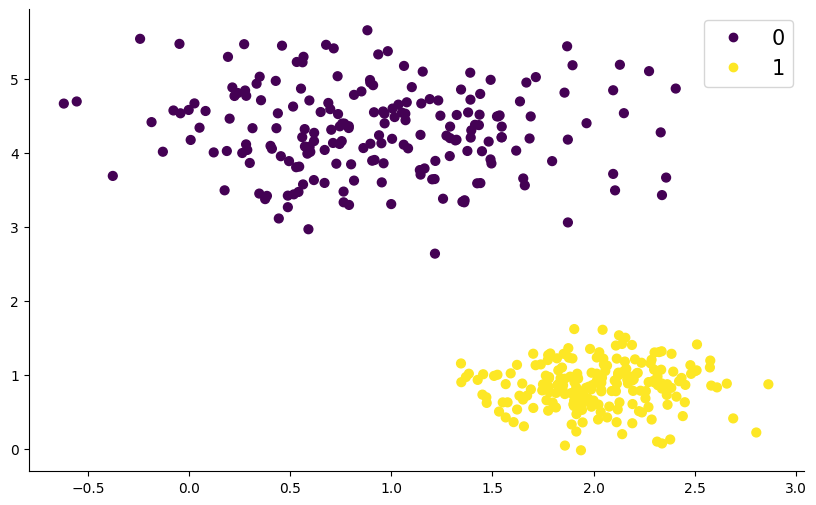
Multivariate Gaussian Mixture Model

Why?

  1. Useful when there are large datasets and it is difficult to find clusters.
  2. More efficient than other clustering algorithms such as k-means.
# imports
import jax
import jax.numpy as jnp
import seaborn as sns
import matplotlib.pyplot as plt
!pip install distrax
import distrax
import tensorflow_probability as tfp
import tensorflow as tf
Collecting distrax
  Downloading distrax-0.1.5-py3-none-any.whl (319 kB)
     ━━━━━━━━━━━━━━━━━━━━━━━━━━━━━━━━━━━━━━━━ 319.7/319.7 kB 5.1 MB/s eta 0:00:00
Requirement already satisfied: absl-py>=0.9.0 in /usr/local/lib/python3.10/dist-packages (from distrax) (1.4.0)
Collecting chex>=0.1.8 (from distrax)
  Downloading chex-0.1.85-py3-none-any.whl (95 kB)
     ━━━━━━━━━━━━━━━━━━━━━━━━━━━━━━━━━━━━━━━━ 95.1/95.1 kB 14.9 MB/s eta 0:00:00
Requirement already satisfied: jax>=0.1.55 in /usr/local/lib/python3.10/dist-packages (from distrax) (0.4.20)
Requirement already satisfied: jaxlib>=0.1.67 in /usr/local/lib/python3.10/dist-packages (from distrax) (0.4.20+cuda11.cudnn86)
Requirement already satisfied: numpy>=1.23.0 in /usr/local/lib/python3.10/dist-packages (from distrax) (1.23.5)
Requirement already satisfied: tensorflow-probability>=0.15.0 in /usr/local/lib/python3.10/dist-packages (from distrax) (0.22.0)
Requirement already satisfied: typing-extensions>=4.2.0 in /usr/local/lib/python3.10/dist-packages (from chex>=0.1.8->distrax) (4.5.0)
Collecting numpy>=1.23.0 (from distrax)
  Downloading numpy-1.26.2-cp310-cp310-manylinux_2_17_x86_64.manylinux2014_x86_64.whl (18.2 MB)
     ━━━━━━━━━━━━━━━━━━━━━━━━━━━━━━━━━━━━━━━━ 18.2/18.2 MB 87.4 MB/s eta 0:00:00
Requirement already satisfied: toolz>=0.9.0 in /usr/local/lib/python3.10/dist-packages (from chex>=0.1.8->distrax) (0.12.0)
Requirement already satisfied: ml-dtypes>=0.2.0 in /usr/local/lib/python3.10/dist-packages (from jax>=0.1.55->distrax) (0.2.0)
Requirement already satisfied: opt-einsum in /usr/local/lib/python3.10/dist-packages (from jax>=0.1.55->distrax) (3.3.0)
Requirement already satisfied: scipy>=1.9 in /usr/local/lib/python3.10/dist-packages (from jax>=0.1.55->distrax) (1.11.3)
Requirement already satisfied: six>=1.10.0 in /usr/local/lib/python3.10/dist-packages (from tensorflow-probability>=0.15.0->distrax) (1.16.0)
Requirement already satisfied: decorator in /usr/local/lib/python3.10/dist-packages (from tensorflow-probability>=0.15.0->distrax) (4.4.2)
Requirement already satisfied: cloudpickle>=1.3 in /usr/local/lib/python3.10/dist-packages (from tensorflow-probability>=0.15.0->distrax) (2.2.1)
Requirement already satisfied: gast>=0.3.2 in /usr/local/lib/python3.10/dist-packages (from tensorflow-probability>=0.15.0->distrax) (0.5.4)
Requirement already satisfied: dm-tree in /usr/local/lib/python3.10/dist-packages (from tensorflow-probability>=0.15.0->distrax) (0.1.8)
Installing collected packages: numpy, chex, distrax
  Attempting uninstall: numpy
    Found existing installation: numpy 1.23.5
    Uninstalling numpy-1.23.5:
      Successfully uninstalled numpy-1.23.5
  Attempting uninstall: chex
    Found existing installation: chex 0.1.7
    Uninstalling chex-0.1.7:
      Successfully uninstalled chex-0.1.7
ERROR: pip's dependency resolver does not currently take into account all the packages that are installed. This behaviour is the source of the following dependency conflicts.
lida 0.0.10 requires fastapi, which is not installed.
lida 0.0.10 requires kaleido, which is not installed.
lida 0.0.10 requires python-multipart, which is not installed.
lida 0.0.10 requires uvicorn, which is not installed.
cupy-cuda11x 11.0.0 requires numpy<1.26,>=1.20, but you have numpy 1.26.2 which is incompatible.
Successfully installed chex-0.1.85 distrax-0.1.5 numpy-1.26.2
from sklearn.datasets import make_blobs
X, y_true = make_blobs(n_samples=400, centers=2,
                       cluster_std=[0.6, 0.3], random_state=0)
plt.figure(figsize=(10, 6))
sc = plt.scatter(X[:, 0], X[:, 1], c=y_true, s=40, cmap='viridis')
plt.legend(*sc.legend_elements(), fontsize=15)
sns.despine()
plt.show()

So if we wanted to find the probability of a point belonging to either of the two clusters, can we directly add the two pdfs? i.e.

\[\begin{equation} P_{1}(X) + P_{2}(X) = P(X)? \end{equation}\]

Answer -> NO!

\[\begin{equation} P_{1}(X) \ and\ P_{2}(X) \end{equation}\] both integrate to 1 so if we add these two we will get a distribution which integrates to 2!
This violates the normalization constraint that the integral of a PDF must be 1 over all domain.

Solution?

Introduce some weighting coefficients in front of the two distributions such that the normalization is not violated. Thus,

\[\begin{equation} P(X) = π_{0}P_{0}(X) + π_{1}P_{1}(X) \end{equation}\]

In general if we have d multivariate gaussian distributions,

\[\begin{equation} P(X) = \sum_{d=0}^{D-1}π_{d}P_{d}(X) \end{equation}\]

One important observation:

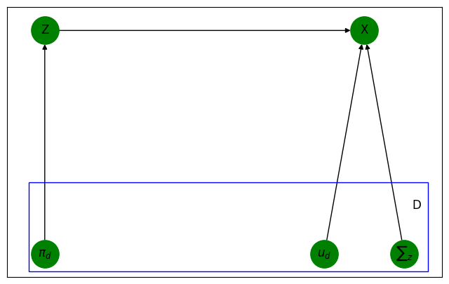
We don’t know to which cluster does a point belong to. We are interested in finding out the same. Hence this is a latent information i.e. the information we don’t observe. Thus \(P(X)\) is a marginal PDF.

Now let us model the clusters as \(Z = {0,......D-1}\), which makes it easy for us to perform cluster assignment. Thus the set \(Z\) determines the position \(X\).

Remember! We don’t observe \(Z\), i.e. we do not know to which cluster does \(X\) belong to.

\[\begin{align} X&\sim MultNormal(X;μ_{z},\Sigma_{z}) \\ Z&\sim Cat(z,π) \end{align}\]

import networkx as nx
import pylab
from matplotlib.patches import Rectangle
fig, my_ax = plt.subplots(figsize=(8, 5))
G = nx.DiGraph()
G.add_edges_from([('Z', 'X'), (r'$π_d$', 'Z'),
                 (r'$u_d$', 'X'), (r'$∑_{z}$', 'X')])
fixed_positions = {'Z': (0, 0), 'X': (2, 0), r'$π_d$': (
    0, -0.25), r'$u_d$': (1.75, -0.25), r'$∑_{z}$': (2.25, -0.25)}
fixed_nodes = fixed_positions.keys()
pos = nx.spring_layout(G, pos=fixed_positions, fixed=fixed_nodes)
nx.draw_networkx(G, with_labels=True, node_color='green',
                 pos=pos, node_size=800)
my_ax.add_patch(Rectangle((-0.1, -0.27), 2.5, 0.1,
                linewidth=1, edgecolor='b', facecolor='none'))
my_ax.text(2.3, -0.2, "D", fontsize=12)
plt.show()

\[\begin{equation} P(Z,X) = P(Z)P(X|Z) \\ = Cat(Z;π)N(X;μ_{z},\Sigma_{z}) \\ = \left(\prod_{d=0}^{D-1} \pi_{d}^{I(z=d)}\right) \frac{1}{\sqrt{(2π)^{k}det\left(\Sigma_{z}\right)}} \exp \left(-\frac{1}{2}\left(x-\mu_{-z}\right)^{\top} \sum^{-1}(x-\mu_{-z})\right) \end{equation}\]

Marginalizing this:

\[\begin{equation} P(X) = \sum_{d=0}^{D-1}p(Z=d,X) \end{equation}\]

image.png

image.png
key = jax.random.PRNGKey(0)
theta = jnp.array([0.5, 0.5])  # probs for s1, s2
mu = jnp.array([[-2.0, -1.0], [2.5, 1.5]])
sigma = jnp.array([[0.5, 0.5], [0.5, 0.5]])
cat = distrax.Categorical(probs=theta)
components = distrax.MultivariateNormalDiag(loc=mu, scale_diag=sigma)

mixture = distrax.MixtureSameFamily(cat, components)
X = mixture.sample(seed=key, sample_shape=1000)
plt.figure(figsize=(10, 6))
plt.scatter(X[:, 0], X[:, 1])
<matplotlib.collections.PathCollection at 0x7e1c40686140>

x_0 = jnp.linspace(-4, 4, 100)
x_1 = jnp.linspace(-4, 4, 100)
X_0, X_1 = jnp.meshgrid(x_0, x_1)
points = jnp.stack((X_0.flatten(), X_1.flatten())).T
prob_at_points = mixture.prob(points)
prob_at_points = prob_at_points.reshape(100, 100)
plt.figure(figsize=(10, 6))
plt.contour(X_0, X_1, prob_at_points)
<matplotlib.contour.QuadContourSet at 0x7e1c40557e50>

Recall

EM(Expectation Maximization) Algorithm -

E step:

\[\begin{equation} γ_{ij} = P(Z=d|X = x^{[i]};θ^{[u]}) \\ \end{equation}\]

M step

\[\begin{equation} θ^{[u+1]} = argmax_{θ} \sum_{i=0}^{N-1}\sum_{d=0}^{D-1}γ_{ij}log(P(Z=d;X = x^{[i]},θ)) \end{equation}\]

This is a constrained optimization problem since these are the two constraints we have:

\[\begin{equation} \sum_{c=0}^{D-1}π_{c} = 1 \end{equation}\]

\[\begin{equation} \sum_{d}>0 (Symmetric \ Positive \ Definite) \end{equation}\]

We use the Lagrangian method to solve for \(π\), \(μ\), \(\Sigma\) and \(λ\).

\[\begin{equation} Q̂(θ,λ) = Q(θ) + λ(1 -\sum_{c=0}^{D-1}π_{c}) \end{equation}\]

Now this is in uncontrained optimization so we can differentiate wrt each of the individual parameters and find the values for maximization.

Solving it we get:
E-step 1. \(γ_{ij}(\text{un-normalized}) = π_{j}N(X = x^{[i]};ν_{j},\sum_{j})\) 2. \(γ_{ij}(\text{normalized}) = \frac{γ_{ij}(\text{un-normalized})}{\sum_{d=0}^{D-1}γ_{id}(\text{un-normalized})}\) 3. \(γ_{j} = \sum_{i=0}^{N-1}γ_{ij}(\text{normalized})\)

M-step: 1. \(π_{j} = \frac{γ_{j}}{N}\) 2. \(ν_{j} = \frac{\sum_{i=0}^{N-1}γ_{ij}X^{[i]}}{γ_{j}}\) 3. \(\sum_{j} = \frac{(X-1ν_{j}^{T})^{T}((X-1ν_{j}^{T}).γ_{j}1_{k}^{T})}{γ_{j}}\)

def em2(dataset, n_clusters, n_iter=100):
    # Infer from the dataset
    n_samples, n_dims = dataset.shape
    # Draw initial guesses
    cluster_probs = tfp.distributions.Dirichlet(
        tf.ones(n_clusters)).sample(seed=42)
    mus = tfp.distributions.Normal(loc=0.0, scale=3.0).sample(
        (n_clusters, n_dims), seed=42)
    covs = tfp.distributions.WishartTriL(
        df=3, scale_tril=tf.eye(n_dims)).sample(n_clusters, seed=42)

    for _ in range(n_iter):
        # Batched Cholesky Factorization
        Ls = tf.linalg.cholesky(covs)
        normals = tfp.distributions.MultivariateNormalTriL(
            loc=mus,
            scale_tril=Ls
        )

        # E-Step

        # (1) resp is of shape (n_samples x n_clusters)
        # batched multivariate normal is of shape (n_clusters x n_dims)
        unnormalized_responsibilities = (
            tf.reshape(cluster_probs, (1, n_clusters)) *
            normals.prob(tf.reshape(dataset, (n_samples, 1, n_dims)))
        )

        # (2)
        responsibilities = unnormalized_responsibilities / \
            tf.reduce_sum(unnormalized_responsibilities, axis=1, keepdims=True)

        # (3)
        class_responsibilities = tf.reduce_sum(responsibilities, axis=0)

        # M-Step
        # (1)
        cluster_probs = class_responsibilities / n_samples

        # (2)
        # class_responsibilities is of shape (n_clusters)
        # responsibilities is of shape (n_samples, n_clusters)
        # dataset is of shape (n_samples, n_dims)
        #
        # mus is of shape (n_clusters, n_dims)
        #
        # -> summation has to occur over the samples axis
        mus = tf.reduce_sum(
            tf.reshape(responsibilities, (n_samples, n_clusters, 1)) *
            tf.reshape(dataset, (n_samples, 1, n_dims)),
            axis=0,
        ) / tf.reshape(class_responsibilities, (n_clusters, 1))

        # (3)
        # class_responsibilities is of shape (n_clusters)
        # dataset is of shape (n_samples, n_dims)
        # mus is of shape (n_clusters, n_dims)
        # responsibilities is of shape (n_samples, n_clusters)
        #
        # covs is of shape (n_clusters, n_dims, n_dims)

        # (n_clusters, n_samples, n_dims)
        centered_datasets = tf.reshape(
            dataset, (1, n_samples, n_dims)) - tf.reshape(mus, (n_clusters, 1, n_dims))
        centered_datasets_with_responsibilities = centered_datasets * \
            tf.reshape(tf.transpose(responsibilities),
                       (n_clusters, n_samples, 1))

        # Batched Matrix Multiplication
        # (n_clusters, n_dims, n_dims)
        sample_covs = tf.matmul(
            centered_datasets_with_responsibilities, centered_datasets, transpose_a=True)

        covs = sample_covs / \
            tf.reshape(class_responsibilities, (n_clusters, 1, 1))

        # Ensure positive definiteness by adding a "small amount" to the diagonal
        covs = covs + 1.0e-8 * tf.eye(n_dims, batch_shape=(n_clusters, ))

    return cluster_probs, mus, covs
key = jax.random.PRNGKey(0)
N_CLUSTERS = 2
N_SAMPLES = 100000
theta = jnp.array([0.3, 0.7])  # probs for s1, s2
mu = jnp.array([[5.0, 5.0], [-3.0, -2.0]])
sigma = jnp.array([[0.5, 0.5], [0.5, 0.5]])
cat = distrax.Categorical(probs=theta)
components = distrax.MultivariateNormalDiag(loc=mu, scale_diag=sigma)
mixture = distrax.MixtureSameFamily(cat, components)
dataset = mixture.sample(seed=key, sample_shape=N_SAMPLES)
class_probs_approx, mus_approx, covs_approx = em2(dataset, N_CLUSTERS)

print("------")
print("Class Probabilities")
print(class_probs_approx)
print("------")
print("Mus")
print(mus_approx)
print("------")
print("Covariance Matrices")
print(covs_approx)
------
Class Probabilities
tf.Tensor([0.69975 0.30025], shape=(2,), dtype=float32)
------
Mus
tf.Tensor(
[[-2.997861  -1.9988518]
 [ 4.9977436  4.9973416]], shape=(2, 2), dtype=float32)
------
Covariance Matrices
tf.Tensor(
[[[ 2.4818128e-01  1.6083641e-04]
  [ 1.6083641e-04  2.4958798e-01]]

 [[ 2.5431883e-01 -2.6203133e-04]
  [-2.6203133e-04  2.5133604e-01]]], shape=(2, 2, 2), dtype=float32)