%%capture
%matplotlib inline
from functools import partial
import matplotlib.pyplot as plt
import math
try:
    import optax
except ModuleNotFoundError:
    %pip install -qq optax
    import optax
import jax
import jax.numpy as jnp
from jax import jit
from jax.nn.initializers import glorot_normal
try:
    import flax
except ModuleNotFoundError:
    %pip install -qq flax
    import flax
import flax.linen as nn
from flax.training import train_state
import tensorflow_probability.substrates.jax as tfp
from typing import Any, Callable, Sequence
import optax

!pip install jaxopt
import jaxopt
import jax
import jax.numpy as jnp
import numpy as np
import tensorflow as tf
from tqdm import tqdm
import seaborn as sns
from flax.core import unfreeze
import randomMotivation
Neural network traditionally give point estimates on the test data. These predictions could be either a guess or be completely wrong. A better approach would be to give a range or a band of predictions instead of one value. This band of predictions can help in making a decision. For example: If I were to predict the AQI measure for city A for tomorrow, an interval \(I\in[200,230]\) is better than a single number like \(195\).
Model architecture and loss function
A neural network model with activation function as RELU (Rectified Linear Unit) to introduce a degree of non-linearity. The loss function is the squared error loss. The architecture is defined by the user.
class load(nn.Module):
    features: list

    @nn.compact
    def __call__(self, X, deterministic, rate=0.03):
        for i, feature in enumerate(self.features):
            X = nn.Dense(feature, name=f"layer{i}")(X)
            if i != 0 and i != len(self.features) - 1:
                X = nn.relu(X)
                X = nn.Dropout(rate=rate, deterministic=deterministic)(X)
        return X

    def loss_fn(self, params, X, y, deterministic=False, key=jax.random.PRNGKey(0)):
        y_pred = self.apply(params, X, False, rngs={"dropout": key})
        loss = jnp.sum((y - y_pred)**2)/(2*X.shape[0])
        return loss
We use a Adam optimizer and use JAX to do the automatic gradient computation using “value_and_grad.” It takes a function and returns a function where the argument specified remains the same for subsequent calls. When the function is called again, further parameters can now be defined which helps increase the flexibility of the code whereas also helps fix particular set of parameters which the user wants should be same across all function calls.
def fit(model, params, X, y, learning_rate=0.01, epochs=100, key=0, verbose=False):
    opt = optax.adam(learning_rate=learning_rate)
    opt_state = opt.init(params)

    loss_grad_fn = jax.jit(jax.value_and_grad(model.loss_fn))
    key = jax.random.PRNGKey(key)
    losses = []
    for i in range(epochs):
        key, _ = jax.random.split(key)
        loss_val, grads = loss_grad_fn(params, X, y, True)
        updates, opt_state = opt.update(grads, opt_state)
        params = optax.apply_updates(params, updates)
        losses.append(loss_val)
        if verbose and i % (epochs / 10) == 0:
            print('Loss step {}: '.format(i), loss_val)
    return params, jnp.array(losses)
In sin data, the noise added is multiplied with \(x\) whereas in hetero data, the noise is multiplied with \(x^2\). Since the noise is dependant on x, it becomes heteroscedastic data.
def data_sin(points=20, xrange=(-3, 3), std=0.3):
    xx = jnp.linspace(-1, 1, 1000).reshape(-1, 1)
    key = jax.random.PRNGKey(0)
    epsilons = jax.random.normal(key, shape=(3,)) * 0.02
    y_true = jnp.array([[x + 0.3 * jnp.sin(2 * jnp.pi * (x + epsilons[0])) +
                       0.3 * jnp.sin(4 * jnp.pi * (x + epsilons[1])) + epsilons[2]] for x in xx])
    yy = jnp.array([[x + 0.3 * jnp.sin(2 * jnp.pi * (x + epsilons[0])) + 0.3 * jnp.sin(4 *
                   jnp.pi * (x + epsilons[1])) + epsilons[2] + x*np.random.normal(0, std)] for x in xx])
    return xx.reshape(1000, 1), yy.reshape(1000, 1), y_true.reshape(1000, 1)


def data_hetero(points=20, xrange=(-3, 3), std=0.3):
    xx = jnp.linspace(-1, 1, 1000).reshape(-1, 1)
    key = jax.random.PRNGKey(0)
    y_true = jnp.array([[x*10*x] for x in xx])
    yy = jnp.array([[x*10*x + x*x*np.random.normal(0, std)] for x in xx])
    return xx.reshape(1000, 1), yy.reshape(1000, 1), y_true.reshape(1000, 1)
key, subkey = jax.random.split(jax.random.PRNGKey(0))
X, Y, y_true = data_sin(points=1000, xrange=(-1, 1), std=2)
plt.figure()
plt.scatter(X, Y, alpha=0.8)
plt.plot(X, y_true, linewidth=2, color='black', linestyle='-')
sns.despine()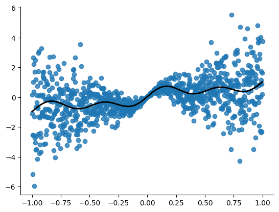
model = load([32, 64, 1])We keep the number of neural networks in the bootstrapping process to be 5. Generally, it can be kept as large as 50 too.
n_estimators = 5
x_grid = jnp.linspace(-2, 2, 1000).reshape(-1, 1)
keys = jax.random.split(jax.random.PRNGKey(0), n_estimators)
Y_final = []
parameters = []
for i in range(n_estimators):
    ids = jax.random.choice(keys[i], jnp.array(range(1000)), (1000, 1))
    x, y = X[ids], Y[ids]
    loss = []
    params = model.init(keys[i], x, True)
    params, losses = fit(model, params, x, y,  epochs=100)
    Y_pred = model.apply(params, x_grid, True)
    parameters.append(params)
    Y_final.append(Y_pred)
Y_final = jnp.array(Y_final)
mean = Y_final.mean(axis=0)
std = Y_final.std(axis=0)
mean = mean.squeeze()
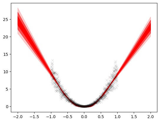
std = std.squeeze()We can see here since the training data lied between \(-1\) and \(1\), the standard deviation did not change much but outside this interval, it increased as x increased. This is the particular characteristic of a bayesian model. If the model gave point predictions, using the error, we would get a constant band of uncertainty i.e. the error itself. This gives no information and does not take into consideration the nature of the model since it is trained on a limited interval and outside these intervals, its uncertainty should naturally increase. This is seen in the bayesian model.
plt.plot(X, Y, 'kx', alpha=0.1)
plt.fill_between(x_grid.squeeze(), mean+std, mean-std, color='red', alpha=1)
plt.fill_between(x_grid.squeeze(), mean+2*std,
                 mean-2*std, color='red', alpha=0.6)
plt.fill_between(x_grid.squeeze(), mean+3*std,
                 mean-3*std, color='red', alpha=0.2)
<matplotlib.collections.PolyCollection at 0x2aad1a58e50>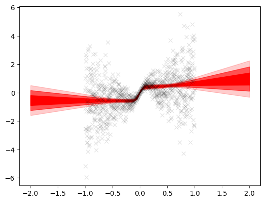
Quadratic dataset
key, subkey = jax.random.split(jax.random.PRNGKey(0))
X, Y, y_true = data_hetero(points=1000, xrange=(-1, 1), std=2)
plt.figure()
plt.scatter(X, Y, alpha=0.8)
plt.plot(X, y_true, linewidth=2, color='black', linestyle='-')
sns.despine()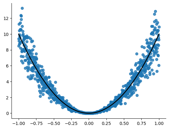
model = load([32, 64, 1])n_estimators = 5
x_grid = jnp.linspace(-2, 2, 1000).reshape(-1, 1)
keys = jax.random.split(jax.random.PRNGKey(0), n_estimators)
Y_final = []
parameters = []
for i in range(n_estimators):
ids = jax.random.choice(keys[i], jnp.array(range(1000)), (1000, 1))
x, y = X[ids], Y[ids]
loss = []
params = model.init(keys[i], x, True)
params, losses = fit(model, params, x, y, epochs=100)
Y_pred = model.apply(params, x_grid, True)
parameters.append(params)
Y_final.append(Y_pred)Y_final = jnp.array(Y_final)
mean = Y_final.mean(axis=0)
std = Y_final.std(axis=0)
mean = mean.squeeze()
std = std.squeeze()Here too the effect is similar as above. Outside \([-1, 1]\), the uncertainty bands increase. However within the training region, the uncertainty band is narrow since the model is more sure about the training predictions.
plt.plot(X, Y, 'kx', alpha=0.1)
plt.fill_between(x_grid.squeeze(), mean+std, mean-std, color='red', alpha=1)
plt.fill_between(x_grid.squeeze(), mean+2*std,
                 mean-2*std, color='red', alpha=0.6)
plt.fill_between(x_grid.squeeze(), mean+3*std,
                 mean-3*std, color='red', alpha=0.2)
<matplotlib.collections.PolyCollection at 0x2aad88c2bc0>