Effect of Dropout on MNIST Classifier

Neural Network without MC Dropout

!pip install -q flax

     |████████████████████████████████| 185 kB 5.3 MB/s 
     |████████████████████████████████| 145 kB 60.2 MB/s 
     |████████████████████████████████| 237 kB 59.4 MB/s 
     |████████████████████████████████| 51 kB 5.8 MB/s 
     |████████████████████████████████| 85 kB 3.4 MB/s 

# necessary imports
import jax
import jax.numpy as jnp
from flax import linen as nn
from flax.training import train_state
import numpy as np
import optax
import tensorflow_datasets as tfds

Architecture: 1. \(32\) neurons 2. \(64\) neurons 3. \(256\) neurons 4. \(10\) output neurons for \(10\) classes

class CNN(nn.Module):
    @nn.compact
    def __call__(self, x, deterministic: bool = True):
        x = nn.Conv(features=32, kernel_size=(3, 3))(x)
        x = nn.relu(x)
        x = nn.avg_pool(x, window_shape=(2, 2), strides=(2, 2))
        x = nn.Conv(features=64, kernel_size=(3, 3))(x)
        x = nn.relu(x)
        x = nn.Dropout(0.3, deterministic=deterministic)(x)
        x = nn.avg_pool(x, window_shape=(2, 2), strides=(2, 2))
        x = x.reshape((x.shape[0], -1))
        x = nn.Dense(features=256)(x)
        x = nn.relu(x)
        x = nn.Dense(features=10)(x)
        return x

# Loss function for multi-class classification = cross-entropy loss
def cross_entropy_loss(*, logits, labels):
    # one-hot encoding for cross entropy loss
    labels_onehot = jax.nn.one_hot(labels, num_classes=10)
    return optax.softmax_cross_entropy(logits=logits, labels=labels_onehot).mean()

# compute-metrics for returning the loss and accuracy of the model
def compute_metrics(*, logits, labels):
    loss = cross_entropy_loss(logits=logits, labels=labels)
    accuracy = jnp.mean(jnp.argmax(logits, -1) == labels)
    metrics = {
        'loss': loss,
        'accuracy': accuracy,
    }
    return metrics

def get_datasets():  # dataset-loader
    ds_builder = tfds.builder('mnist')
    ds_builder.download_and_prepare()
    train_ds = tfds.as_numpy(
        ds_builder.as_dataset(split='train', batch_size=-1))
    test_ds = tfds.as_numpy(ds_builder.as_dataset(split='test', batch_size=-1))
    train_ds['image'] = jnp.float32(train_ds['image']) / 255.
    test_ds['image'] = jnp.float32(test_ds['image']) / 255.
    return train_ds, test_ds

def create_train_state(rng, learning_rate, momentum):
    cnn = CNN()  # model initialized
    init_rng = {'params': rng, 'dropout': jax.random.PRNGKey(10)}
    params = cnn.init(rng, jnp.ones([1, 28, 28, 1]))['params']
    # Stochastic gradient descent for params
    tx = optax.sgd(learning_rate, momentum)
    return train_state.TrainState.create(apply_fn=cnn.apply, params=params, tx=tx)

@jax.jit
def train_step(state, batch):
    def loss_fn(params, rngs):  # training for a single step
        logits = CNN().apply({'params': params},
                             batch['image'], deterministic=True, rngs=rngs)
        loss = cross_entropy_loss(logits=logits, labels=batch['label'])
        return loss, logits
    grad_fn = jax.value_and_grad(loss_fn, has_aux=True)
    (_, logits), grads = grad_fn(state.params,
                                 rngs={'dropout': jax.random.PRNGKey(0)})
    state = state.apply_gradients(grads=grads)
    metrics = compute_metrics(logits=logits, labels=batch['label'])
    return state, metrics

@jax.jit  # gives the loss and accuracy of the model on the test images
def eval_step(params, batch):
    logits = CNN().apply({'params': params}, batch['image'], deterministic=True, rngs={
        'dropout': jax.random.PRNGKey(0)})
    return compute_metrics(logits=logits, labels=batch['label']), logits

def train_epoch(state, train_ds, batch_size, epoch, rng):  # Train for a single epoch
    train_size = len(train_ds['image'])
    steps_per_epoch = train_size // batch_size
    perms = jax.random.permutation(rng, train_size)
    # in case of incomplete batch since no. of training points might not be a clear multiple of the batch size
    perms = perms[:steps_per_epoch * batch_size]
    perms = perms.reshape((steps_per_epoch, batch_size))
    batch_metrics = []
    for perm in perms:
        batch = {k: v[perm, ...] for k, v in train_ds.items()}
        state, metrics = train_step(state, batch)
        batch_metrics.append(metrics)

    batch_metrics_np = jax.device_get(batch_metrics)
    epoch_metrics_np = {
        k: np.mean([metrics[k] for metrics in batch_metrics_np])
        for k in batch_metrics_np[0]}

    print('train epoch: %d, loss: %.4f, accuracy: %.2f' %
          (epoch, epoch_metrics_np['loss'], epoch_metrics_np['accuracy'] * 100))
    return state

def eval_model(params, test_ds):
    metrics, logits = eval_step(params, test_ds)
    logits = jax.device_get(logits)
    metrics = jax.device_get(metrics)
    summary = jax.tree_util.tree_map(lambda x: x.item(), metrics)
    return summary['loss'], summary['accuracy'], logits

train_ds, test_ds = get_datasets()  # get the datasets

rng = jax.random.PRNGKey(0)
rng, init_rng = jax.random.split(rng)

learning_rate = 0.1
momentum = 0.9

state = create_train_state(init_rng, learning_rate, momentum)
del init_rng  # Must not be used anymore.

num_epochs = 10
batch_size = 32

import jax
import jax.numpy as jnp

We iterate through the original dataset which is in the form of a dictionary with the keys as images and labels respectively. Then by running a simple for loop, we add the images and the corresponding labels to the \(x\) and \(y\) arrays. Since we need \(500\) images of each class, we stop if the count of the images left to be added becomes zero. After the loop, \(500\) images of each class has been added to the two arrays for training and further evaluation.

count_train = [500]*10
x_train_final = np.empty([5000, 28, 28, 1])
y_train_final = np.empty([5000,])
j = 0
for i in range(6000):
    if (train_ds['label'][i] == 0 and count_train[0] > 0):
        x_train_final[j] = train_ds['image'][j]
        y_train_final[j] = train_ds['label'][j]
        count_train[0] -= 1
        j += 1
    if (train_ds['label'][i] == 1 and count_train[1] > 0):
        x_train_final[j] = train_ds['image'][j]
        y_train_final[j] = train_ds['label'][j]
        count_train[1] -= 1
        j += 1
    if (train_ds['label'][i] == 2 and count_train[2] > 0):
        x_train_final[j] = train_ds['image'][j]
        y_train_final[j] = train_ds['label'][j]
        count_train[2] -= 1
        j += 1
    if (train_ds['label'][i] == 3 and count_train[3] > 0):
        x_train_final[j] = train_ds['image'][j]
        y_train_final[j] = train_ds['label'][j]
        count_train[3] -= 1
        j += 1
    if (train_ds['label'][i] == 4 and count_train[4] > 0):
        x_train_final[j] = train_ds['image'][j]
        y_train_final[j] = train_ds['label'][j]
        count_train[4] -= 1
        j += 1
    if (train_ds['label'][i] == 5 and count_train[5] > 0):
        x_train_final[j] = train_ds['image'][j]
        y_train_final[j] = train_ds['label'][j]
        count_train[5] -= 1
        j += 1
    if (train_ds['label'][i] == 6 and count_train[6] > 0):
        x_train_final[j] = train_ds['image'][j]
        y_train_final[j] = train_ds['label'][j]
        count_train[6] -= 1
        j += 1

    if (train_ds['label'][i] == 7 and count_train[7] > 0):
        x_train_final[j] = train_ds['image'][j]
        y_train_final[j] = train_ds['label'][j]
        count_train[7] -= 1
        j += 1

    if (train_ds['label'][i] == 8 and count_train[8] > 0):
        x_train_final[j] = train_ds['image'][j]
        y_train_final[j] = train_ds['label'][j]
        count_train[8] -= 1
        j += 1

    if (train_ds['label'][i] == 9 and count_train[9] > 0):
        x_train_final[j] = train_ds['image'][j]
        y_train_final[j] = train_ds['label'][j]
        count_train[9] -= 1
        j += 1

After the loop, \(100\) images of each class has been added to the two arrays for testing and further evaluation.

count_test = [100]*10
x_test_final = np.empty([1000, 28, 28, 1])
y_test_final = np.empty([1000,])
j = 0
for i in range(1300):
    if (test_ds['label'][i] == 0 and count_test[0] > 0):
        x_test_final[j] = test_ds['image'][j]
        y_test_final[j] = test_ds['label'][j]
        count_test[0] -= 1
        j += 1
    if (test_ds['label'][i] == 1 and count_test[1] > 0):
        x_test_final[j] = test_ds['image'][j]
        y_test_final[j] = test_ds['label'][j]
        count_test[1] -= 1
        j += 1
    if (test_ds['label'][i] == 2 and count_test[2] > 0):
        x_test_final[j] = test_ds['image'][j]
        y_test_final[j] = test_ds['label'][j]
        count_test[2] -= 1
        j += 1
    if (test_ds['label'][i] == 3 and count_test[3] > 0):
        x_test_final[j] = test_ds['image'][j]
        y_test_final[j] = test_ds['label'][j]
        count_test[3] -= 1
        j += 1
    if (test_ds['label'][i] == 4 and count_test[4] > 0):
        x_test_final[j] = test_ds['image'][j]
        y_test_final[j] = test_ds['label'][j]
        count_test[4] -= 1
        j += 1
    if (test_ds['label'][i] == 5 and count_test[5] > 0):
        x_test_final[j] = test_ds['image'][j]
        y_test_final[j] = test_ds['label'][j]
        count_test[5] -= 1
        j += 1
    if (test_ds['label'][i] == 6 and count_test[6] > 0):
        x_test_final[j] = test_ds['image'][j]
        y_test_final[j] = test_ds['label'][j]
        count_test[6] -= 1
        j += 1

    if (test_ds['label'][i] == 7 and count_test[7] > 0):
        x_test_final[j] = test_ds['image'][j]
        y_test_final[j] = test_ds['label'][j]
        count_test[7] -= 1
        j += 1

    if (test_ds['label'][i] == 8 and count_test[8] > 0):
        x_test_final[j] = test_ds['image'][j]
        y_test_final[j] = test_ds['label'][j]
        count_test[8] -= 1
        j += 1

    if (test_ds['label'][i] == 9 and count_test[9] > 0):
        x_test_final[j] = test_ds['image'][j]
        y_test_final[j] = test_ds['label'][j]
        count_test[9] -= 1
        j += 1

Making it in a dictionary format for the evaluation purposes

train_ds_new = {}
train_ds_new['image'] = jnp.array(x_train_final)
train_ds_new['label'] = y_train_final
test_ds_new = {}
test_ds_new['image'] = jnp.array(x_test_final)
test_ds_new['label'] = y_test_final

logits_tot = []
for epoch in range(1, num_epochs + 1):
    rng, input_rng = jax.random.split(rng)
    state = train_epoch(state, train_ds_new, batch_size, epoch, input_rng)
    test_loss, test_accuracy, logits = eval_model(state.params, test_ds_new)
    logits_tot.append(logits)
    print(' test epoch: %d, loss: %.2f, accuracy: %.2f' % (
        epoch, test_loss, test_accuracy * 100))

train epoch: 1, loss: 0.5284, accuracy: 82.71
 test epoch: 1, loss: 0.16, accuracy: 95.10
train epoch: 2, loss: 0.1579, accuracy: 95.01
 test epoch: 2, loss: 0.16, accuracy: 95.40
train epoch: 3, loss: 0.0963, accuracy: 96.96
 test epoch: 3, loss: 0.12, accuracy: 96.10
train epoch: 4, loss: 0.0727, accuracy: 97.56
 test epoch: 4, loss: 0.13, accuracy: 96.30
train epoch: 5, loss: 0.0529, accuracy: 98.16
 test epoch: 5, loss: 0.09, accuracy: 97.50
train epoch: 6, loss: 0.0505, accuracy: 98.44
 test epoch: 6, loss: 0.10, accuracy: 96.80
train epoch: 7, loss: 0.0287, accuracy: 99.02
 test epoch: 7, loss: 0.15, accuracy: 96.10
train epoch: 8, loss: 0.0309, accuracy: 98.94
 test epoch: 8, loss: 0.09, accuracy: 97.70
train epoch: 9, loss: 0.0239, accuracy: 99.32
 test epoch: 9, loss: 0.08, accuracy: 98.10
train epoch: 10, loss: 0.0060, accuracy: 99.76
 test epoch: 10, loss: 0.09, accuracy: 97.90

We can see that in the first training epoch, the accuracy on train and test are good but not upto the level. As the training goes on, the accuracy improves for both the instances. Also the accuracy does not immediately go to \(100\%\) which might become a measure of overfitting if it did so. But here that is not the case.

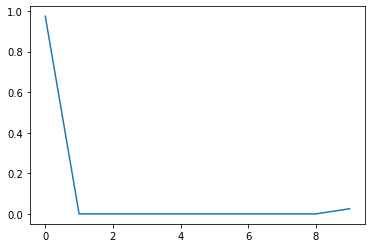
b = nn.softmax(logits_tot[9][-11])

import matplotlib.pyplot as plt
digits = np.arange(10)
plt.plot(digits, b)

def get_datasets_fashion():  # Load MNIST train and test datasets into memory
    ds_builder = tfds.builder('fashion_mnist')
    ds_builder.download_and_prepare()
    train_ds = tfds.as_numpy(
        ds_builder.as_dataset(split='train', batch_size=-1))
    test_ds = tfds.as_numpy(ds_builder.as_dataset(split='test', batch_size=-1))
    train_ds['image'] = jnp.float32(train_ds['image']) / 255.
    test_ds['image'] = jnp.float32(test_ds['image']) / 255.
    return train_ds, test_ds

train_ds_fashion, test_ds_fashion = get_datasets_fashion()

After the loop, \(100\) images of each class has been added to the two arrays for testing and further evaluation.

count_test_fashion = [100]*10
x_test_final_fashion = np.empty([1000, 28, 28, 1])
y_test_final_fashion = np.empty([1000,])
j = 0
for i in range(1300):
    if (test_ds_fashion['label'][i] == 0 and count_test_fashion[0] > 0):
        x_test_final_fashion[j] = test_ds_fashion['image'][j]
        y_test_final_fashion[j] = test_ds_fashion['label'][j]
        count_test_fashion[0] -= 1
        j += 1
    if (test_ds_fashion['label'][i] == 1 and count_test_fashion[1] > 0):
        x_test_final_fashion[j] = test_ds_fashion['image'][j]
        y_test_final_fashion[j] = test_ds_fashion['label'][j]
        count_test_fashion[1] -= 1
        j += 1
    if (test_ds_fashion['label'][i] == 2 and count_test_fashion[2] > 0):
        x_test_final_fashion[j] = test_ds_fashion['image'][j]
        y_test_final_fashion[j] = test_ds_fashion['label'][j]
        count_test_fashion[2] -= 1
        j += 1
    if (test_ds_fashion['label'][i] == 3 and count_test_fashion[3] > 0):
        x_test_final_fashion[j] = test_ds_fashion['image'][j]
        y_test_final_fashion[j] = test_ds_fashion['label'][j]
        count_test_fashion[3] -= 1
        j += 1
    if (test_ds_fashion['label'][i] == 4 and count_test_fashion[4] > 0):
        x_test_final_fashion[j] = test_ds_fashion['image'][j]
        y_test_final_fashion[j] = test_ds_fashion['label'][j]
        count_test_fashion[4] -= 1
        j += 1
    if (test_ds_fashion['label'][i] == 5 and count_test_fashion[5] > 0):
        x_test_final_fashion[j] = test_ds_fashion['image'][j]
        y_test_final_fashion[j] = test_ds_fashion['label'][j]
        count_test_fashion[5] -= 1
        j += 1
    if (test_ds_fashion['label'][i] == 6 and count_test_fashion[6] > 0):
        x_test_final_fashion[j] = test_ds_fashion['image'][j]
        y_test_final_fashion[j] = test_ds_fashion['label'][j]
        count_test_fashion[6] -= 1
        j += 1

    if (test_ds_fashion['label'][i] == 7 and count_test_fashion[7] > 0):
        x_test_final_fashion[j] = test_ds_fashion['image'][j]
        y_test_final_fashion[j] = test_ds_fashion['label'][j]
        count_test_fashion[7] -= 1
        j += 1

    if (test_ds_fashion['label'][i] == 8 and count_test_fashion[8] > 0):
        x_test_final_fashion[j] = test_ds_fashion['image'][j]
        y_test_final_fashion[j] = test_ds_fashion['label'][j]
        count_test[8] -= 1
        j += 1

    if (test_ds_fashion['label'][i] == 9 and count_test[9] > 0):
        x_test_final_fashion[j] = test_ds_fashion['image'][j]
        y_test_final_fashion[j] = test_ds_fashion['label'][j]
        count_test[9] -= 1
        j += 1

test_ds_new_fashion = {}
test_ds_new_fashion['image'] = jnp.array(x_test_final_fashion)
test_ds_new_fashion['label'] = y_test_final_fashion

train_ds_new['image'].shape

(5000, 28, 28, 1)

test_ds_new_fashion['label'].shape

(1000,)

logits = CNN().apply({'params': state.params}, test_ds_new_fashion['image'], deterministic=True, rngs={
    'dropout': jax.random.PRNGKey(0)})
logits = nn.softmax(logits)

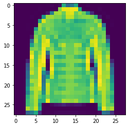
import matplotlib.pyplot as plt
plt.imshow(test_ds_new_fashion['image'][1].reshape(28, 28))

<matplotlib.image.AxesImage at 0x7f4ca5e07750>

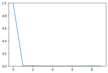
b = logits[1]

import matplotlib.pyplot as plt
digits = np.arange(10)
plt.plot(digits, b)
plt.ylim(0, 1)

(0.0, 1.0)

test_ds_new_fashion['label'][1]

4.0

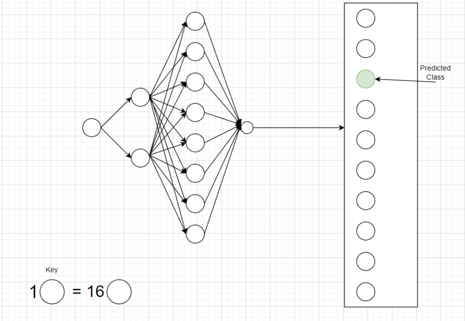
\(99.1\%\) probability! The model is absolutely certain that the image is some digit. This is a big disadvantage of neural networks. Hence we need to incorporate the concept of uncertainty to show us how the much is the model unceratain about its predictions. We use MC Dropout for the next question to show this.

Neural Network with MC Dropout

!pip install -q flax

# necessary imports
import jax
import jax.numpy as jnp
from flax import linen as nn
from flax.training import train_state
import numpy as np
import optax
import tensorflow_datasets as tfds

Architecture: 1. \(32\) neurons 2. \(64\) neurons 3. \(256\) neurons 4. \(10\) output neurons for \(10\) classes

class CNN(nn.Module):
    @nn.compact
    def __call__(self, x, deterministic: bool = True):
        x = nn.Conv(features=32, kernel_size=(3, 3))(x)
        x = nn.relu(x)
        x = nn.avg_pool(x, window_shape=(2, 2), strides=(2, 2))
        x = nn.Conv(features=64, kernel_size=(3, 3))(x)
        x = nn.relu(x)
        x = nn.Dropout(0.3, deterministic=deterministic)(x)
        x = nn.avg_pool(x, window_shape=(2, 2), strides=(2, 2))
        x = x.reshape((x.shape[0], -1))
        x = nn.Dense(features=256)(x)
        x = nn.relu(x)
        x = nn.Dropout(0.3, deterministic=deterministic)(x)
        x = nn.Dense(features=10)(x)
        return x

# Loss function for multi-class classification = cross-entropy loss
def cross_entropy_loss(*, logits, labels):
    # one-hot encoding for cross entropy loss
    labels_onehot = jax.nn.one_hot(labels, num_classes=10)
    return optax.softmax_cross_entropy(logits=logits, labels=labels_onehot).mean()

# compute-metrics for returning the loss and accuracy of the model
def compute_metrics(*, logits, labels):
    loss = cross_entropy_loss(logits=logits, labels=labels)
    accuracy = jnp.mean(jnp.argmax(logits, -1) == labels)
    metrics = {
        'loss': loss,
        'accuracy': accuracy,
    }
    return metrics

def get_datasets():  # dataset-loader
    ds_builder = tfds.builder('mnist')
    ds_builder.download_and_prepare()
    train_ds = tfds.as_numpy(
        ds_builder.as_dataset(split='train', batch_size=-1))
    test_ds = tfds.as_numpy(ds_builder.as_dataset(split='test', batch_size=-1))
    train_ds['image'] = jnp.float32(train_ds['image']) / 255.
    test_ds['image'] = jnp.float32(test_ds['image']) / 255.
    return train_ds, test_ds

def create_train_state(rng, learning_rate, momentum):
    cnn = CNN()  # model initialized
    init_rng = {'params': rng, 'dropout': jax.random.PRNGKey(10)}
    params = cnn.init(rng, jnp.ones([1, 28, 28, 1]))['params']
    # Stochastic gradient descent for params
    tx = optax.sgd(learning_rate, momentum)
    return train_state.TrainState.create(apply_fn=cnn.apply, params=params, tx=tx)

@jax.jit
def train_step(state, batch):
    def loss_fn(params, rngs):  # training for a single step
        logits = CNN().apply({'params': params},
                             batch['image'], deterministic=False, rngs=rngs)
        loss = cross_entropy_loss(logits=logits, labels=batch['label'])
        return loss, logits
    grad_fn = jax.value_and_grad(loss_fn, has_aux=True)
    (_, logits), grads = grad_fn(state.params,
                                 rngs={'dropout': jax.random.PRNGKey(0)})
    state = state.apply_gradients(grads=grads)
    metrics = compute_metrics(logits=logits, labels=batch['label'])
    return state, metrics

@jax.jit  # gives the loss and accuracy of the model on the test images
def eval_step(params, batch):
    logits = CNN().apply({'params': params}, batch['image'], deterministic=False, rngs={
        'dropout': jax.random.PRNGKey(0)})
    return compute_metrics(logits=logits, labels=batch['label']), logits

def train_epoch(state, train_ds, batch_size, epoch, rng):  # Train for a single epoch
    train_size = len(train_ds['image'])
    steps_per_epoch = train_size // batch_size
    perms = jax.random.permutation(rng, train_size)
    # in case of incomplete batch since no. of training points might not be a clear multiple of the batch size
    perms = perms[:steps_per_epoch * batch_size]
    perms = perms.reshape((steps_per_epoch, batch_size))
    batch_metrics = []
    for perm in perms:
        batch = {k: v[perm, ...] for k, v in train_ds.items()}
        state, metrics = train_step(state, batch)
        batch_metrics.append(metrics)

    batch_metrics_np = jax.device_get(batch_metrics)
    epoch_metrics_np = {
        k: np.mean([metrics[k] for metrics in batch_metrics_np])
        for k in batch_metrics_np[0]}

    print('train epoch: %d, loss: %.4f, accuracy: %.2f' %
          (epoch, epoch_metrics_np['loss'], epoch_metrics_np['accuracy'] * 100))
    return state

def eval_model(params, test_ds):
    metrics, logits = eval_step(params, test_ds)
    logits = jax.device_get(logits)
    metrics = jax.device_get(metrics)
    summary = jax.tree_util.tree_map(lambda x: x.item(), metrics)
    return summary['loss'], summary['accuracy'], logits

train_ds, test_ds = get_datasets()  # get the datasets

WARNING:absl:No GPU/TPU found, falling back to CPU. (Set TF_CPP_MIN_LOG_LEVEL=0 and rerun for more info.)

rng = jax.random.PRNGKey(0)
rng, init_rng = jax.random.split(rng)

learning_rate = 0.1
momentum = 0.9

state = create_train_state(init_rng, learning_rate, momentum)
del init_rng  # Must not be used anymore.

num_epochs = 10
batch_size = 32

import jax
import jax.numpy as jnp

We iterate through the original dataset which is in the form of a dictionary with the keys as images and labels respectively. Then by running a simple for loop, we add the images and the corresponding labels to the \(x\) and \(y\) arrays. Since we need 500 images of each class, we stop if the count of the images left to be added becomes zero. After the loop, \(500\) images of each class has been added to the two arrays for training and further evaluation.

count_train = [500]*10
x_train_final = np.empty([5000, 28, 28, 1])
y_train_final = np.empty([5000,])
j = 0
for i in range(6000):
    if (train_ds['label'][i] == 0 and count_train[0] > 0):
        x_train_final[j] = train_ds['image'][j]
        y_train_final[j] = train_ds['label'][j]
        count_train[0] -= 1
        j += 1
    if (train_ds['label'][i] == 1 and count_train[1] > 0):
        x_train_final[j] = train_ds['image'][j]
        y_train_final[j] = train_ds['label'][j]
        count_train[1] -= 1
        j += 1
    if (train_ds['label'][i] == 2 and count_train[2] > 0):
        x_train_final[j] = train_ds['image'][j]
        y_train_final[j] = train_ds['label'][j]
        count_train[2] -= 1
        j += 1
    if (train_ds['label'][i] == 3 and count_train[3] > 0):
        x_train_final[j] = train_ds['image'][j]
        y_train_final[j] = train_ds['label'][j]
        count_train[3] -= 1
        j += 1
    if (train_ds['label'][i] == 4 and count_train[4] > 0):
        x_train_final[j] = train_ds['image'][j]
        y_train_final[j] = train_ds['label'][j]
        count_train[4] -= 1
        j += 1
    if (train_ds['label'][i] == 5 and count_train[5] > 0):
        x_train_final[j] = train_ds['image'][j]
        y_train_final[j] = train_ds['label'][j]
        count_train[5] -= 1
        j += 1
    if (train_ds['label'][i] == 6 and count_train[6] > 0):
        x_train_final[j] = train_ds['image'][j]
        y_train_final[j] = train_ds['label'][j]
        count_train[6] -= 1
        j += 1

    if (train_ds['label'][i] == 7 and count_train[7] > 0):
        x_train_final[j] = train_ds['image'][j]
        y_train_final[j] = train_ds['label'][j]
        count_train[7] -= 1
        j += 1

    if (train_ds['label'][i] == 8 and count_train[8] > 0):
        x_train_final[j] = train_ds['image'][j]
        y_train_final[j] = train_ds['label'][j]
        count_train[8] -= 1
        j += 1

    if (train_ds['label'][i] == 9 and count_train[9] > 0):
        x_train_final[j] = train_ds['image'][j]
        y_train_final[j] = train_ds['label'][j]
        count_train[9] -= 1
        j += 1

After the loop, \(100\) images of each class has been added to the two arrays for testing and further evaluation.

count_test = [100]*10
x_test_final = np.empty([1000, 28, 28, 1])
y_test_final = np.empty([1000,])
j = 0
for i in range(1300):
    if (test_ds['label'][i] == 0 and count_test[0] > 0):
        x_test_final[j] = test_ds['image'][j]
        y_test_final[j] = test_ds['label'][j]
        count_test[0] -= 1
        j += 1
    if (test_ds['label'][i] == 1 and count_test[1] > 0):
        x_test_final[j] = test_ds['image'][j]
        y_test_final[j] = test_ds['label'][j]
        count_test[1] -= 1
        j += 1
    if (test_ds['label'][i] == 2 and count_test[2] > 0):
        x_test_final[j] = test_ds['image'][j]
        y_test_final[j] = test_ds['label'][j]
        count_test[2] -= 1
        j += 1
    if (test_ds['label'][i] == 3 and count_test[3] > 0):
        x_test_final[j] = test_ds['image'][j]
        y_test_final[j] = test_ds['label'][j]
        count_test[3] -= 1
        j += 1
    if (test_ds['label'][i] == 4 and count_test[4] > 0):
        x_test_final[j] = test_ds['image'][j]
        y_test_final[j] = test_ds['label'][j]
        count_test[4] -= 1
        j += 1
    if (test_ds['label'][i] == 5 and count_test[5] > 0):
        x_test_final[j] = test_ds['image'][j]
        y_test_final[j] = test_ds['label'][j]
        count_test[5] -= 1
        j += 1
    if (test_ds['label'][i] == 6 and count_test[6] > 0):
        x_test_final[j] = test_ds['image'][j]
        y_test_final[j] = test_ds['label'][j]
        count_test[6] -= 1
        j += 1

    if (test_ds['label'][i] == 7 and count_test[7] > 0):
        x_test_final[j] = test_ds['image'][j]
        y_test_final[j] = test_ds['label'][j]
        count_test[7] -= 1
        j += 1

    if (test_ds['label'][i] == 8 and count_test[8] > 0):
        x_test_final[j] = test_ds['image'][j]
        y_test_final[j] = test_ds['label'][j]
        count_test[8] -= 1
        j += 1

    if (test_ds['label'][i] == 9 and count_test[9] > 0):
        x_test_final[j] = test_ds['image'][j]
        y_test_final[j] = test_ds['label'][j]
        count_test[9] -= 1
        j += 1

Making it in a dictionary format for the evaluation purposes

train_ds_new = {}
train_ds_new['image'] = jnp.array(x_train_final)
train_ds_new['label'] = y_train_final
test_ds_new = {}
test_ds_new['image'] = jnp.array(x_test_final)
test_ds_new['label'] = y_test_final

logits_tot = []
for epoch in range(1, num_epochs + 1):
    rng, input_rng = jax.random.split(rng)
    state = train_epoch(state, train_ds_new, batch_size, epoch, input_rng)
    test_loss, test_accuracy, logits = eval_model(state.params, test_ds_new)
    logits_tot.append(logits)
    print(' test epoch: %d, loss: %.2f, accuracy: %.2f' % (
        epoch, test_loss, test_accuracy * 100))

train epoch: 1, loss: 0.6127, accuracy: 79.71
 test epoch: 1, loss: 0.37, accuracy: 89.00
train epoch: 2, loss: 0.2125, accuracy: 94.01
 test epoch: 2, loss: 0.25, accuracy: 93.80
train epoch: 3, loss: 0.1559, accuracy: 95.51
 test epoch: 3, loss: 0.27, accuracy: 92.50
train epoch: 4, loss: 0.1685, accuracy: 95.23
 test epoch: 4, loss: 0.22, accuracy: 94.00
train epoch: 5, loss: 0.0978, accuracy: 96.98
 test epoch: 5, loss: 0.17, accuracy: 94.90
train epoch: 6, loss: 0.0954, accuracy: 96.85
 test epoch: 6, loss: 0.19, accuracy: 94.40
train epoch: 7, loss: 0.0942, accuracy: 97.14
 test epoch: 7, loss: 0.17, accuracy: 95.40
train epoch: 8, loss: 0.0648, accuracy: 97.98
 test epoch: 8, loss: 0.14, accuracy: 96.30
train epoch: 9, loss: 0.0713, accuracy: 97.58
 test epoch: 9, loss: 0.18, accuracy: 95.50
train epoch: 10, loss: 0.0464, accuracy: 98.52
 test epoch: 10, loss: 0.15, accuracy: 96.10

We can see that in the first training epoch, the accuracy on train and test are good but not upto the level. As the training goes on, the accuracy improves for both the instances. Also the accuracy does not immediately go to \(100\%\) which might become a measure of overfitting if it did so. But here that is not the case.

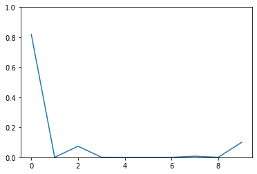
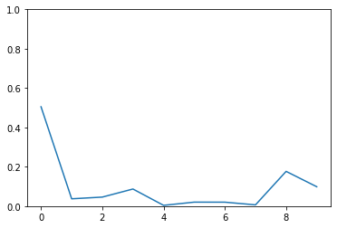
b = nn.softmax(logits_tot[9][-11])

import matplotlib.pyplot as plt
digits = np.arange(10)
plt.plot(digits, b)
plt.ylim(0, 1)

(0.0, 1.0)

def get_datasets_fashion():  # Load MNIST train and test datasets into memory
    ds_builder = tfds.builder('fashion_mnist')
    ds_builder.download_and_prepare()
    train_ds = tfds.as_numpy(
        ds_builder.as_dataset(split='train', batch_size=-1))
    test_ds = tfds.as_numpy(ds_builder.as_dataset(split='test', batch_size=-1))
    train_ds['image'] = jnp.float32(train_ds['image']) / 255.
    test_ds['image'] = jnp.float32(test_ds['image']) / 255.
    return train_ds, test_ds

train_ds_fashion, test_ds_fashion = get_datasets_fashion()

After the loop, \(100\) images of each class has been added to the two arrays for testing and further evaluation.

count_test_fashion = [100]*10
x_test_final_fashion = np.empty([1000, 28, 28, 1])
y_test_final_fashion = np.empty([1000,])
j = 0
for i in range(1300):
    if (test_ds_fashion['label'][i] == 0 and count_test_fashion[0] > 0):
        x_test_final_fashion[j] = test_ds_fashion['image'][j]
        y_test_final_fashion[j] = test_ds_fashion['label'][j]
        count_test_fashion[0] -= 1
        j += 1
    if (test_ds_fashion['label'][i] == 1 and count_test_fashion[1] > 0):
        x_test_final_fashion[j] = test_ds_fashion['image'][j]
        y_test_final_fashion[j] = test_ds_fashion['label'][j]
        count_test_fashion[1] -= 1
        j += 1
    if (test_ds_fashion['label'][i] == 2 and count_test_fashion[2] > 0):
        x_test_final_fashion[j] = test_ds_fashion['image'][j]
        y_test_final_fashion[j] = test_ds_fashion['label'][j]
        count_test_fashion[2] -= 1
        j += 1
    if (test_ds_fashion['label'][i] == 3 and count_test_fashion[3] > 0):
        x_test_final_fashion[j] = test_ds_fashion['image'][j]
        y_test_final_fashion[j] = test_ds_fashion['label'][j]
        count_test_fashion[3] -= 1
        j += 1
    if (test_ds_fashion['label'][i] == 4 and count_test_fashion[4] > 0):
        x_test_final_fashion[j] = test_ds_fashion['image'][j]
        y_test_final_fashion[j] = test_ds_fashion['label'][j]
        count_test_fashion[4] -= 1
        j += 1
    if (test_ds_fashion['label'][i] == 5 and count_test_fashion[5] > 0):
        x_test_final_fashion[j] = test_ds_fashion['image'][j]
        y_test_final_fashion[j] = test_ds_fashion['label'][j]
        count_test_fashion[5] -= 1
        j += 1
    if (test_ds_fashion['label'][i] == 6 and count_test_fashion[6] > 0):
        x_test_final_fashion[j] = test_ds_fashion['image'][j]
        y_test_final_fashion[j] = test_ds_fashion['label'][j]
        count_test_fashion[6] -= 1
        j += 1

    if (test_ds_fashion['label'][i] == 7 and count_test_fashion[7] > 0):
        x_test_final_fashion[j] = test_ds_fashion['image'][j]
        y_test_final_fashion[j] = test_ds_fashion['label'][j]
        count_test_fashion[7] -= 1
        j += 1

    if (test_ds_fashion['label'][i] == 8 and count_test_fashion[8] > 0):
        x_test_final_fashion[j] = test_ds_fashion['image'][j]
        y_test_final_fashion[j] = test_ds_fashion['label'][j]
        count_test[8] -= 1
        j += 1

    if (test_ds_fashion['label'][i] == 9 and count_test[9] > 0):
        x_test_final_fashion[j] = test_ds_fashion['image'][j]
        y_test_final_fashion[j] = test_ds_fashion['label'][j]
        count_test[9] -= 1
        j += 1

test_ds_new_fashion = {}
test_ds_new_fashion['image'] = jnp.array(x_test_final_fashion)
test_ds_new_fashion['label'] = y_test_final_fashion

train_ds_new['image'].shape

(5000, 28, 28, 1)

test_ds_new_fashion['label'].shape

(1000,)

logits = CNN().apply({'params': state.params}, test_ds_new_fashion['image'], deterministic=False, rngs={
    'dropout': jax.random.PRNGKey(0)})
logits = nn.softmax(logits)

import matplotlib.pyplot as plt
plt.imshow(test_ds_new_fashion['image'][1].reshape(28, 28))

<matplotlib.image.AxesImage at 0x7f65ee417b10>

b = logits[1]

import matplotlib.pyplot as plt
digits = np.arange(10)
plt.plot(digits, b)
plt.ylim(0, 1)

(0.0, 1.0)

b

DeviceArray([0.50489163, 0.03711339, 0.04582743, 0.08685064, 0.00386149,
             0.0201791 , 0.01996568, 0.00632725, 0.1765369 , 0.09844656],            dtype=float32)

test_ds_new_fashion['label'][1]

4.0

\(50\%\) probability! The model is now uncertain about its prediction. This is a big advantage of MC Dropout. Here we have incorporated the concept of uncertainty to show us how the much is the model unceratain about its predictions. Although the prediction is wrong, \(50\%\) probability shows that it is uncertain.